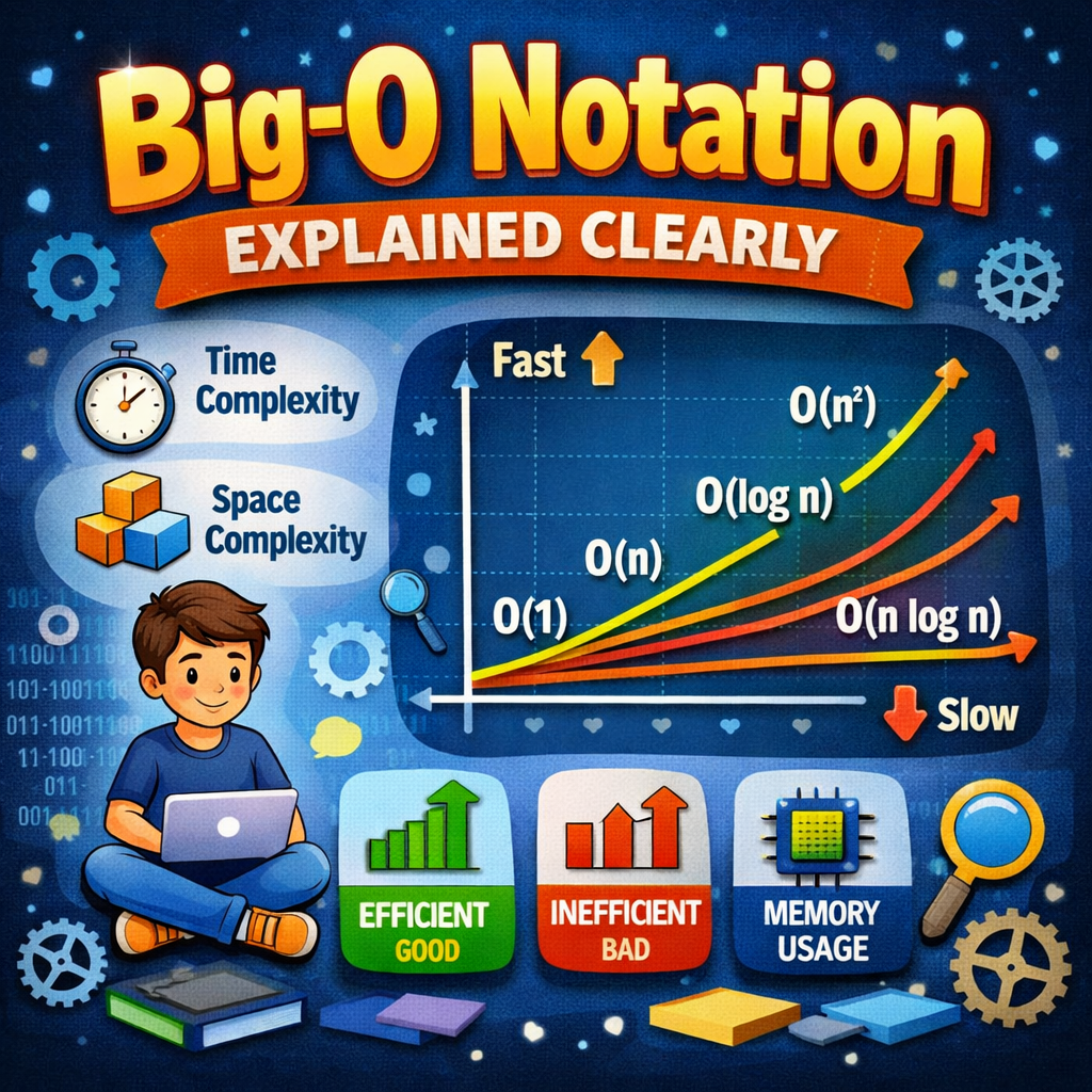
Big-O notation measures how an algorithm performs as input size grows. It helps you understand whether your code will scale or fail under heavy load.
- O(1) → constant time (fastest)
- O(log n) → very efficient
- O(n) → linear growth
- O(n²) → slow for large inputs
If two solutions solve the same problem, Big-O tells you which one survives in production.
A Simple Story Before We Start
You build a feature that searches for users in a database.
During testing, it works instantly. There are only 100 users.
Then your product grows. Now there are 10 lakh users.
Suddenly:
- Search takes seconds
- CPU usage spikes
- Users complain
You didn’t change the code. So, what has changed?
Input size.
Your algorithm that worked fine for 100 users is now inefficient for 1,000,000 users.
This is where Big-O notation becomes critical.
Because in real systems, the question is not: “Does it work?”
The real question is: “Will it still work when data grows?”
What is Big-O Notation?
Big-O notation describes how the time or space required by an algorithm grows with input size (n).
It does not measure exact time. It measures growth behavior.
For example:
- Does your algorithm double in time when input doubles?
- Or does it increase slowly?
Big-O answers this.
Why Big-O Matters in Real Systems
In production systems:
- Data grows continuously
- Users increase
- Requests scale
An inefficient algorithm may:
- Crash systems
- Increase latency
- Consume unnecessary resources
Efficient algorithms ensure:
- Fast responses
- Low resource usage
- Better scalability
This is why companies care deeply about algorithm efficiency.
Master DSA for top tech interviews
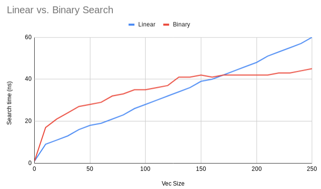
Understanding Growth with an Example
Let’s compare two approaches to find an element in an array.
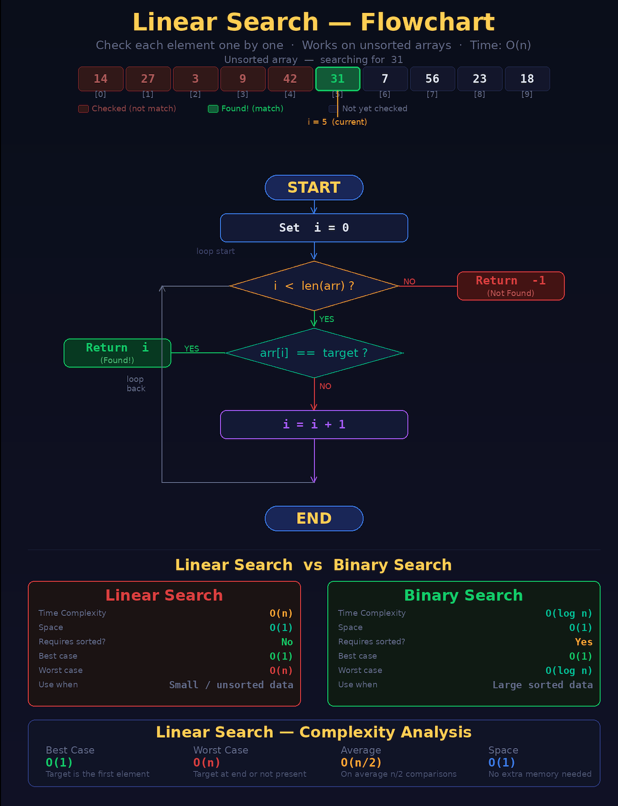
Approach 1 – Linear Search
for(int i = 0; i < n; i++){
    if(arr[i] == target){
        return i;
    }
}
Time complexity: O(n)
You may check every element.
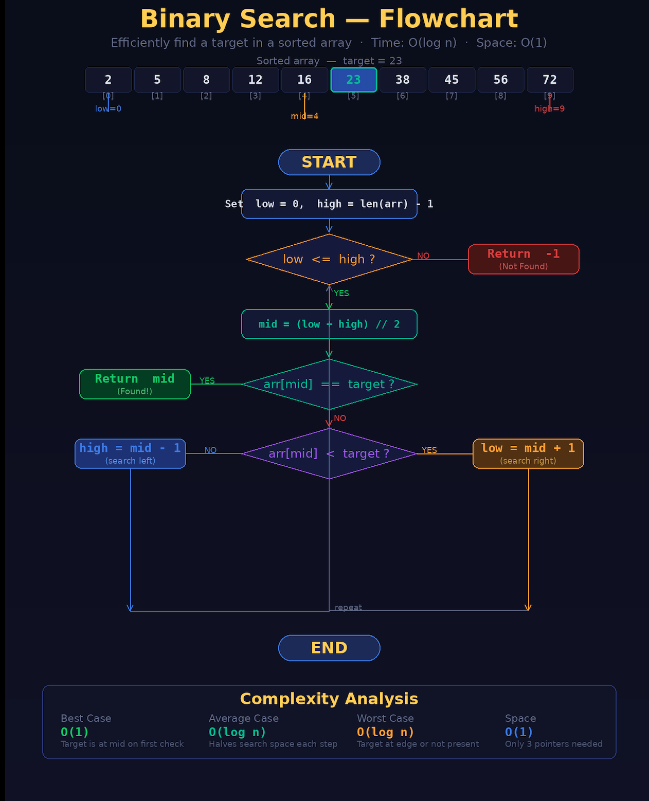
Approach 2 – Binary Search (sorted array)
while(left <= right){
    int mid = (left + right) / 2;

    if(arr[mid] == target) return mid;
    else if(arr[mid] < target) left = mid + 1;
    else right = mid - 1;
}
Time complexity: O(log n)
Each step cuts the search space in half.
Even though both solve the same problem, their performance differs drastically at scale.
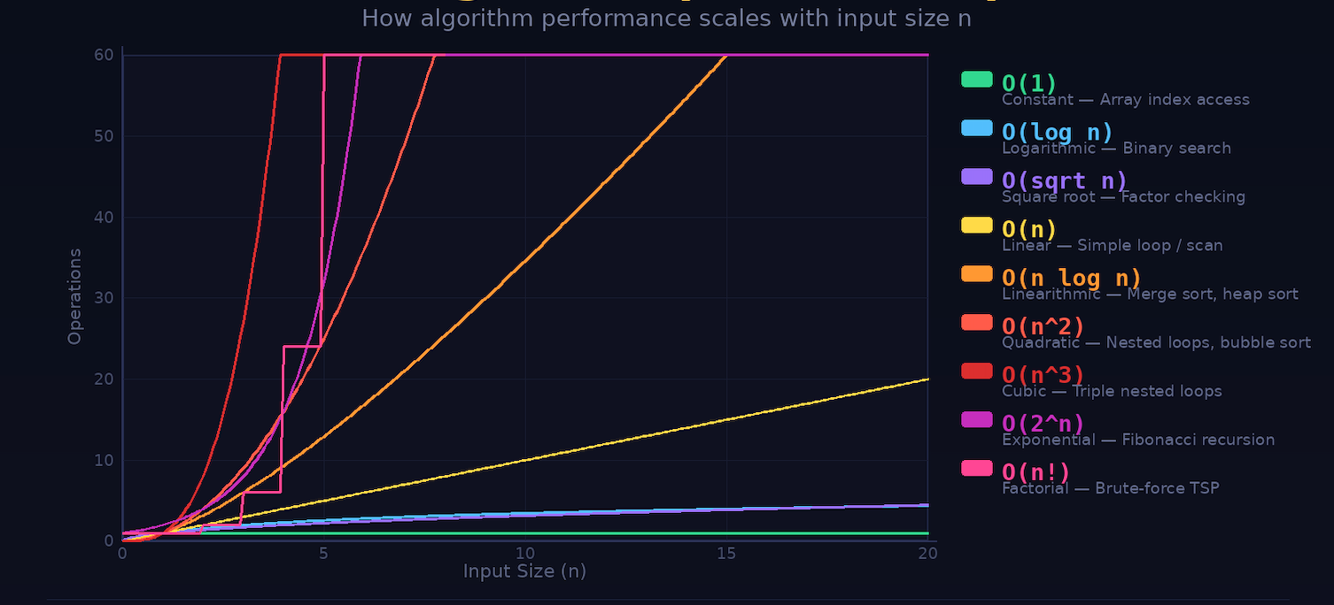
Common Big-O Complexities Explained
| Algorithm | Best Time Complexity | Average Time Complexity | Worst Time Complexity | Worst Space Complexity |
|---|---|---|---|---|
| Linear Search | O(1) | O(n) | O(n) | O(1) |
| Binary Search | O(1) | O(log n) | O(log n) | O(1) |
| Bubble Sort | O(n) | O(n²) | O(n²) | O(1) |
| Selection Sort | O(n²) | O(n²) | O(n²) | O(1) |
| Insertion Sort | O(n) | O(n²) | O(n²) | O(1) |
| Merge Sort | O(n log n) | O(n log n) | O(n log n) | O(n) |
| Quick Sort | O(n log n) | O(n log n) | O(n²) | O(log n) |
| Heap Sort | O(n log n) | O(n log n) | O(n log n) | O(n) |
| Bucket Sort | O(n+k) | O(n+k) | O(n²) | O(n) |
| Radix Sort | O(nk) | O(nk) | O(nk) | O(n+k) |
| Tim Sort | O(n) | O(n log n) | O(n log n) | O(n) |
| Shell Sort | O(n) | O((n log(n))²) | O((n log(n))²) | O(1) |
O(1) – Constant Time
The operation takes the same time regardless of input size.
int x = arr[5];Even if array size grows, access time remains constant.
O(log n) – Logarithmic Time
The input size reduces drastically in each step.
Example:
- Binary Search
Efficient even for very large data.
O(n) – Linear Time
Time increases proportionally with input size.
for(int i = 0; i < n; i++){
    // operation
}
O(n log n)
Common in efficient sorting algorithms.
Example:
- Merge Sort
- Quick Sort
O(n²) – Quadratic Time
Nested loops usually lead to this.
for(int i = 0; i < n; i++){
    for(int j = 0; j < n; j++){
        // operation
    }
}
This becomes very slow as input grows.
Time Complexity vs Space Complexity
Big-O is not just about time. It also measures space (memory usage).
Time Complexity
How long does an algorithm takes to execute.
Space Complexity
How much memory an algorithm uses.
int[] temp = new int[n];This adds O(n) space complexity.
Trade-Off Between Time and Space
Sometimes:
- Faster algorithms use more memory
- Memory-efficient algorithms take more time
Example:
- HashMap → fast lookup (O(1)) but uses extra space
- Loop search → less memory but slower (O(n))
Choosing the right balance is key in system design.
How to Analyze Time Complexity
When reading code, look for:
1. Loops
- Single loop → O(n)
- Nested loop → O(n²)
2. Recursion
Depends on how many times function calls itself.
3. Divide and Conquer
Algorithms that reduce problem size:
→ Usually O(log n) or O(n log n)
Real-World Examples
Big-O is everywhere in real systems.
Search engines
Efficient indexing avoids scanning billions of pages linearly.
E-commerce platforms
Sorting products must be fast even with large inventories.
Navigation systems
Pathfinding algorithms must compute routes quickly.
Social media feeds
Ranking algorithms must handle massive data in real time.
Design scalable systems used by top companies
Common Mistakes Beginners Make
- Focusing only on correctness, not efficiency
- Ignoring input size impact
- Not recognizing nested loops
- Overusing brute-force approaches
Correct code is not enough. Efficient code is what matters in production.
A Simple Rule to Remember
If input size grows:
- Good algorithms scale smoothly
- Bad algorithms collapse
Big-O helps you identify the difference early.
Frequently Asked Questions (FAQ)
Is Big-O only for interviews?
No. It is critical for real-world system performance.
Do small projects need Big-O?
Not always, but understanding it early prevents bad habits.
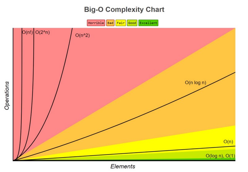
Which complexity is best?
- O(1) is ideal
- O(log n) is very efficient
- O(n) is acceptable
- O(n²) should be avoided for large inputs
Is Big-O difficult to learn?
No. It becomes intuitive with practice and examples.
Final Thoughts
In modern systems, performance is not optional.
Users expect speed. Systems must handle scale. Data continues to grow.
Big-O notation gives you a way to predict performance before problems occur.
It helps you write code that is not just correct, but efficient, scalable, and production ready.
And that is what separates:
- someone who writes code
- someone who engineers systems
Ready to see Big-O thinking in a real system? Read how Tinder matches millions of users in milliseconds – and the algorithm decisions behind it.